Connect with us

Economics

US House of Representatives election: live results

Published

on

On November 5th America will pick its next president, as well as the House of Representatives and a third of the Senate. The Economist will publish live results and analysis covering every race. Check back here soon after first polls close at 6pm EST / 11pm GMT to see in real-time how many votes Kamala Harris and Donald Trump are picking up, and which of them will win the White House, as well as which party will control the two chambers of Congress.

Before then, this page provides a guide for what to look out for ahead of the election. Elsewhere, our daily updated election forecasts calculate each presidential candidate’s chances of winning, and who might take the House and the Senate. Our poll tracker rounds up the latest presidential polls. And The US in brief, our daily update delivered by newsletter, gives you all the election stories that matter.

What to watch

This year, given large numbers of people have voted early, many expect the counting will be slow. Officials, however, insist that ballot tallying will be faster than in previous years. The results could be known just a few hours after polls close across the country—as they were for seven of the past ten elections (see chart). Or they could take days to become clear.

The first states to conclude voting will be on the east coast. Six states, including the key battleground of Georgia, will finish voting statewide at 7pm EST. By 8pm, 19 more states will have joined them and a flurry of data will be published. Readers should exercise caution: little of substance will be revealed at this stage of the night, unless the election is a landslide.

In some states, where one candidate is heavily favoured, the election result will be called almost immediately. Unless there is a major upset or a striking trend, these calls may not say much about the election overall. The absence of a call may be more informative: it may indicate that an expected landslide has not happened, for instance.

The final result will probably come down to seven key states. Of those, Georgia and Michigan may be the fastest to count. North Carolina is also traditionally quick to count but may experience disruption due to Hurricane Helene.

Others could well be slower. Pennsylvania will not start processing millions of postal ballots until the morning of election day. Arizona and Nevada, in the west, finish voting later that day and take longer to count their mail-in ballots, which are popular in both states. Nevada accepts and counts ballots which arrive after election day, too (although these are unlikely to flip the state).

Read more about what to watch on the night, and in the days that follow.

What are the candidates’ paths to victory?

Pennsylvania is the most important state for both candidates. (Mr Trump won Pennsylvania in 2016, but it flipped to Joe Biden in 2020.) According to our forecast model, as of November 4th, Ms Harris wins in 92% of our simulations when she takes the Keystone State’s 19 electoral votes; Mr Trump wins in 88%.

Mr Trump has even better odds when he wins Michigan (95%), but he has more alternative routes to the presidency without Michigan than without Pennsylvania. Other swing states are less influential: Ms Harris and Mr Trump win the election in only 71% and 67% of simulations, respectively, when they win Nevada, a state with only six electoral votes.

The most likely outcome—occurring in 19% of our simulated elections on November 4th—is that Mr Trump will win all seven swing states and go on to win the presidency. The second-most likely is the exact opposite: our model gave Ms Harris a 9% chance of sweeping the seven. The third would give all of the swing states except Nevada to Mr Trump—that would be a repeat of the 2016 result. But based on all of our model’s scenarios, the race is a toss-up: neither candidate has a lead big enough to offset the kind of polling errors seen in previous presidential elections.

Continue Reading

Economics

U.S.- Canada Trade Talks Collapse; Carney Says Retaliatory Tariffs Begin September 8

Published

on

U.S.- Canada Trade Talks Collapse; Carney Says Retaliatory Tariffs Begin September 8

Trade negotiations between the United States and Canada collapsed this week, with Canadian Prime Minister Mark Carney announcing that retaliatory tariffs on U.S. goods will take effect September 8, 2026. The breakdown follows the Trump administration’s imposition of 50% tariffs on certain Canadian goods, according to reporting from CNBC and the Washington Post.

What Happened

CNBC reported the collapse of talks as part of its ongoing business news coverage on August 22, 2026, noting the story as one of the week’s most significant developments for cross-border trade. The Washington Post’s business desk, in coverage also published August 22-23, quoted Carney characterizing President Trump’s 50% tariffs as “a miscalculation,” and confirmed the September 8 date for Canada’s retaliatory measures.

As of this writing, specific details on which categories of U.S. goods will be subject to Canadian retaliatory tariffs have not been fully reported. This article will be updated with additional specifics as they become available from primary government sources.

Why This Matters for Markets and Consumers

Trade disputes between the U.S. and its largest trading partners tend to have ripple effects across supply chains, consumer prices, and specific industry sectors with cross-border exposure. A Washington Post analysis accompanying the coverage noted that other countries unhappy with existing U.S. trade arrangements are likely watching the U.S.-Canada breakdown closely, suggesting the dispute could have implications beyond the immediate bilateral relationship.

Broader Context: A Volatile Week for Cross-Border and Fiscal News

The trade breakdown arrived during an already turbulent week for U.S. economic news. The same week saw the national debt cross $40 trillion for the first time, a sharp rise in Treasury bond market volatility, and the Treasury Department doubling the size of its debt buyback program. Whether the trade dispute has any direct connection to these fiscal and monetary developments has not been established in current reporting, but the concentration of major economic stories in the same week has drawn attention from market commentators tracking overall macroeconomic risk.

How This Fits the Broader Trade Policy Pattern

The U.S.-Canada breakdown is not occurring in isolation. Trade policy has been an active area of U.S. economic policymaking throughout 2026, with tariff actions and negotiations affecting multiple trading partners over the course of the year. Canada has historically been among the United States’ largest trading partners by total trade volume, meaning a prolonged dispute carries more direct economic exposure for both economies than a similar breakdown with a smaller trading partner would.

Industries with integrated North American supply chains — including automotive manufacturing, agriculture, and energy — have historically been among the most exposed to U.S.-Canada trade friction, given the degree to which components and raw materials cross the border multiple times during production. Businesses in these sectors should treat the September 8 deadline as a planning point regardless of whether it ultimately takes effect as announced.

What We Don’t Yet Know

Several material details remain unconfirmed or unreported as of this writing:

– The specific list of U.S. product categories subject to Canadian retaliatory tariffs
– Whether any further negotiations are scheduled between the September 8 deadline and the present
– Potential exemptions for critical supply chains, such as energy or auto parts, which have historically received special treatment in prior U.S.-Canada trade disputes

What to Watch Next

Businesses with cross-border exposure to Canadian suppliers or customers should monitor official statements from the U.S. Trade Representative’s office and Canada’s Department of Global Affairs for detailed tariff schedules ahead of the September 8 implementation date. Given the fluid nature of trade negotiations, a resumption of talks or a modified agreement before that date remains possible and would supersede current retaliatory tariff plans.

Continue Reading

Economics

U.S. National Debt Surpasses $40 Trillion for the First Time: What It Means for the Economy

Published

on

US Debt is now 40 trillions

The U.S. gross national debt crossed $40 trillion for the first time this week, according to Treasury Department data reported by NPR on August 20, 2026. The milestone caps a period of rapid fiscal expansion: the debt has doubled since 2017, and the federal government now spends more than $1 trillion a year just servicing interest on what it owes.

Why the Debt Load Is Accelerating

The debt has not grown at a steady pace. Instead, a combination of pandemic-era spending, tax policy changes, and elevated interest rates has compounded the federal government’s borrowing costs. As older Treasury bonds issued at lower rates mature, they are being refinanced at today’s higher prevailing rates, which pushes up the government’s annual interest bill even without any new borrowing.

That interest bill is no longer a minor line item. At more than $1 trillion annually, debt servicing now competes directly with discretionary spending on defense, infrastructure, and social programs. Economists watching the trend note that this dynamic can become self-reinforcing: higher interest costs widen the deficit, which requires more borrowing, which in turn raises future interest costs.

Bond Market Reaction

The debt milestone arrived during a volatile week for Treasury bonds. Bond prices fell even as equity markets touched record highs, a divergence that market analysts describe as bond investors signaling concern about the sustainability of federal borrowing, even as stock investors remain focused on corporate earnings and AI-driven growth.

U.S. Treasury Secretary Scott Bessent responded to the bond market pressure by expanding the Treasury’s debt buyback program, telling CNBC the size of buyback operations had been doubled to at least $4 billion per operation, with room to increase further. Buybacks are intended to support demand for existing Treasury securities and help stabilize yields during periods of market stress.

What Rising Debt Means for Ordinary Households

For everyday consumers, the national debt level itself is abstract, but its downstream effects are not. Elevated Treasury yields tend to push up borrowing costs across the economy, including mortgage rates, auto loans, and business credit. The same week the $40 trillion milestone was confirmed, average 30-year mortgage rates moved sharply, illustrating how bond market volatility connects directly to household borrowing costs.

Rising federal interest costs also narrow the government’s fiscal flexibility. As a larger share of the federal budget goes toward servicing debt rather than funding programs, policymakers face growing pressure to either cut spending, raise revenue, or both — choices that carry direct economic consequences for households and businesses alike.

What to Watch Next

The debt trajectory is expected to remain a central topic at the Federal Reserve’s Jackson Hole Economic Symposium, scheduled for August 27–29, 2026 — the first such gathering under new Fed Chair Kevin Warsh, who was confirmed by the Senate in a 54-45 vote in May 2026. While the symposium’s stated theme is financial innovation and payments policy, fiscal sustainability and its interaction with monetary policy are likely to feature in sideline discussions given the scale of the debt milestone.

Investors and households should watch upcoming Treasury auction results and any further changes to the buyback program as early indicators of how markets are digesting the government’s borrowing needs. A weak auction — one that requires higher yields to attract sufficient buyers — would be a signal that investor appetite for U.S. debt is softening further.

The $40 trillion figure is a threshold, not a crisis in itself. But combined with a bond market already showing signs of strain, it adds urgency to a fiscal conversation that has largely been deferred by successive Congresses and administrations.

Continue Reading

Economics

Economic Profile of the United States of America (2026–2030 Horizon)

Published

on

Economic Profile of the United States of America (2026–2030 Horizon)

Executive Summary & Core Macro Outlook

The United States enters the 2026–2030 macroeconomic window as the unquestioned heavyweight of nominal economic output, retaining its status as the primary engine of global financial liquidity, private enterprise innovation, and high-margin technological deployment. According to multi-year projections from the International Monetary Fund (IMF) World Economic Outlook and complementary datasets from the World Bank, the US nominal Gross Domestic Product (GDP) is projected to reach $32.38 trillion by 2026, accounting for approximately 25% of global nominal output and roughly 14.5% of world GDP measured at Purchasing Power Parity (PPP).

Unlike many of its advanced-economy peers across Western Europe and East Asia—which are grappling with acute demographic contraction and structural energy shocks—the United States demonstrates remarkable macroeconomic resilience. The IMF projects a real GDP Compound Annual Growth Rate (CAGR) of 2.1% to 2.3% through 2030. This expansion is sustained by three structural anchors: unmatched capital depth driving massive private-sector investment in Artificial Intelligence (AI) infrastructure, complete energy independence as a net exporter of hydrocarbons and liquefied natural gas (LNG), and high labor productivity gains that cushion the economy against rising debt-servicing costs.

Macroeconomic Data Matrix (2026–2030 Projections)

Economic MetricIMF / World Bank Baseline (2026–2030)Global Benchmark & Context
Nominal GDP (2026 Projection)~$32.38 TrillionRank #1 Globally
GDP at Purchasing Power Parity (PPP)~$32.40 TrillionRank #2 Globally (Behind China’s ~$38.5T PPP)
Projected Real GDP CAGR (2026–2030)2.1% – 2.3%Top decile among G7 advanced economies
Gross Public Debt (% of GDP)~122.5% – 128.0%Structural fiscal deficit trajectory
Core Inflation Rate (PCE Target)Stabilizing at 2.0% – 2.2%Federal Reserve inflation target alignment
Current Account Balance (% of GDP)-2.8% to -3.2%Persistent capital import & reserve currency demand

Deep Structural Growth Drivers

1. The AI Infrastructure Hyper-Cycle & TFP Expansion

The defining growth catalyst for the US economy over the 2026–2030 horizon is the unprecedented scale of private capital expenditure (Capex) poured into artificial intelligence infrastructure, enterprise software integration, and advanced computing hardware.

Major technology mega-caps and private equity funds are directing hundreds of billions of dollars annually into hyper-scale data centers, domestic semiconductor fabrication, high-voltage electrical grid upgrades, and AI-driven workflow platforms. According to World Bank economic research, technological adoption across American service and manufacturing sectors is driving a notable uptick in Total Factor Productivity (TFP). This productivity surge allows US companies to expand profit margins and output even in an environment characterized by higher structural real interest rates and tight skilled-labor markets.

2. Deep Capital Markets and Private Sector Liquidity

The structural backbone of US economic outperformance remains its financial system. US capital markets represent over 40% of global equity market capitalization and a vast majority of global venture capital and private credit assets.

This liquidity creates an efficient mechanism for capital allocation: high-potential emerging industries (such as quantum computing, synthetic biology, and advanced defense technology) receive early-stage funding at a scale that no other national market can match. When global monetary conditions tighten, global capital flees toward safety and yield, reinforcing US capital depth and lowering the relative cost of equity capital for American corporations.

3. Net Energy Independence & Industrial Cost Advantages

Unlike industrial hubs in Germany, Japan, or South Korea—which remain highly vulnerable to volatile sea-lane logistics and imported fuel price spikes—the United States operates as a major net exporter of petroleum, natural gas, and refined chemical products.

Access to abundant, cheap domestic natural gas provides US heavy industry, advanced manufacturing, and electricity-hungry data centers with a persistent structural cost advantage. Furthermore, federal policy frameworks (including the CHIPS and Science Act and clean energy tax provisions) continue to catalyze domestic private manufacturing investment, re-shoring high-value supply chains from East Asia back to the American Sunbelt and Midwest.

Macroeconomic Vulnerabilities & Downside Risks

1. Structural Sovereign Debt Trajectory

The most significant medium-term threat to US macroeconomic stability is the path of federal public debt. With gross national debt exceeding 120% of GDP and annual federal deficits running between 5% and 7% of GDP, the US fiscal baseline faces increasing structural pressure.

As older legacy low-yield Treasury bonds mature, they are refinanced at higher prevailing interest rates. According to IMF fiscal monitor assessments, federal net interest payments are absorbing an expanding share of total fiscal revenue, crowding out discretionary spending and narrowing the government’s capacity to deploy counter-cyclical fiscal stimulus during future downturns.

2. Commercial Real Estate (CRE) & Banking Sector Realignment

The structural transformation toward hybrid work models has permanently altered office space utilization across major US metropolitan areas. Regional and community banks, which hold a disproportionate share of commercial real estate debt, face ongoing balance-sheet pressure as legacy office loans mature and require refinancing at lower property valuations and higher interest rates. While systemic money-center banks remain well-capitalized, localized credit tightening from regional lenders presents a headwind for small-and-medium enterprise (SME) borrowing.

High-Outperformance Sector Matrix (2026–2030)
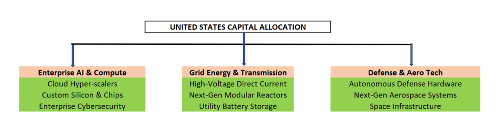
                     
  1. Enterprise AI, Cloud Compute, & Cybersecurity: Companies building enterprise-grade software, AI agents, cloud architectures, and specialized hardware protection layers.
  2. Next-Generation Energy & Grid Modernization: Power generation utilities, high-voltage electrical equipment makers, small modular nuclear reactor (SMR) developers, and energy storage systems catering to exponential data center energy demands.
  3. Advanced Defense Technology & Aerospace: Autonomous systems, satellite networks, hypersonic defense, and advanced materials supplying both domestic security needs and global allied demand.

Strategic Summary for Global Investors & Executives

The United States through 2030 remains the ultimate high-volume, high-yield destination for institutional capital. While fiscal debt risks require long-term monitoring, the immediate 5-year outlook is defined by strong technology-driven productivity, resilient private consumption, and unmatched market liquidity. For global corporations and institutional allocators, exposure to the US economy remains an indispensable pillar of long-term growth strategy.

Top 65 Largest Economies in the World for 2027

Top 10 Largest Economies by 2030: IMF & World Bank GDP Projections for Global Powerhouses

Continue Reading

Trending