
Economics
Why Kamala Harris’s chances of victory just jumped


The Economist’s statistical model of America’s presidential election will be updated six more times before votes are counted. There are few opportunities for candidates to move the dial in an election which has been stubbornly close since Kamala Harris became the Democratic nominee. Today’s update will cheer her supporters: the vice-president’s probability of victory rose by six percentage points, making the race a dead heat.
There are three reasons. One is the volume of new polls—65 were added to our forecast today—giving the model more confidence about small changes. Another is that there is so little time left before the election. Up until now our model has been a forecast, with weeks or months left for candidates to make gains. Many pollsters are now publishing their final surveys of the cycle, so the forecast will soon become a “now-cast”.

The third is that the race is remarkably close, which means that even tiny changes in expected vote shares can yield large shifts in win probabilities. The most influential polls yesterday were concentrated in four states: Michigan, North Carolina, Pennsylvania and Wisconsin. In those states, Ms Harris’s forecasted vote share rose by an average of 0.4 percentage points (see chart)—a small move that was nonetheless sufficient to increase her chance of victory by an average of six percentage points across the four.
On the surface, the new polls did not look unusually good for Ms Harris. Most showed results that were close to a tie. However, the firms that released surveys yesterday—particularly AtlasIntel, Quantus and Trafalgar—have tended to give Donald Trump better numbers this year than have other pollsters who surveyed the same races at similar times. Our model shifts all poll results to counteract such biases. And on average, these adjustments nudged vote margins in yesterday’s swing-state polls around half a percentage point in Ms Harris’s direction.

Moreover, in recent days the model has been moving towards Mr Trump, and Ms Harris’s average projected vote share (excluding third parties) had fallen below 50% in every swing state besides Michigan. As a result, new polls showing a tied race (like those in Pennsylvania did on average after our adjustments) or even a slim lead for Mr Trump (as did those in North Carolina) still represented an improvement for Ms Harris, compared with the model’s relatively gloomy expectations for her yesterday.
New polls also came out in Arizona and Georgia yesterday with a wide spread of results, ranging from an eight-point lead for Mr Trump to a one-point edge for Ms Harris. However, after our adjustments, the average of these new surveys landed very close to the model’s previous expectation of a two-point lead for Mr Trump in both states. As a result, the forecasts for Arizona and Georgia were unchanged.
Ms Harris’s small gains have brought her back to parity in Nevada, Pennsylvania and Wisconsin and made her a narrow favourite in Michigan, whereas Mr Trump retains a small but clear edge in Arizona, Georgia and North Carolina. The two candidates each won exactly half of our model’s simulations in its latest run. On average, they both wind up with 269 electoral votes—which would leave the House of Representatives to break the tie, presumably in Mr Trump’s favour. However, the model assigns just a 1% chance to an actual electoral-college tie, which would probably require Ms Harris to win Michigan, Pennsylvania and Wisconsin while losing Nebraska’s second Congressional district.
The direction or size of polling errors cannot be predicted. But if history is any guide, surveys are likely to underestimate one candidate by a margin that dwarfs the small day-to-day shifts in our model’s average estimates. Any such error would probably deliver a decisive victory to whichever candidate it benefits. Despite the tight polls, our forecast gives a two-in-five chance of the winning candidate receiving more electoral votes than Joe Biden did in 2020 or Mr Trump did in 2016.
The other main source of uncertainty in our model, aside from polling errors, is the time remaining until the election. The forecast works by estimating the candidates’ current positions with the available data, and then simulating movement that could occur each day until November 5th. With just six remaining, there is little movement left to make.
The effect on our forecasted probabilities is counterintuitive. There are few opportunities for big changes in public opinion, meaning polls published now have greater weight. As a result, the forecasted probabilities may change more substantially from day to day than they would earlier in the cycle. The slight movement in Ms Harris’s favour today is harder to reverse in the next six days than it would have been a month ago.
The polls in today’s forecast update were mostly based on interviews conducted a few days ago, so it is hard to judge what, if anything, caused a small uptick in Ms Harris’s standing. Some polls now being published were conducted after Mr Trump’s rally at Madison Square Garden on October 27th—which is now roundly considered to have been a misstep for his campaign—but it is unlikely to be until after the election that we have a clear idea of whether that event moved many voters. It appears as though the final six days of the campaign will go in a similar fashion to the past three months: plenty to talk about, but no decisive leader. ■













Economics
U.S. National Debt Surpasses $40 Trillion for the First Time: What It Means for the Economy



Executive Summary & Core Macro Outlook
The United States enters the 2026–2030 macroeconomic window as the unquestioned heavyweight of nominal economic output, retaining its status as the primary engine of global financial liquidity, private enterprise innovation, and high-margin technological deployment. According to multi-year projections from the International Monetary Fund (IMF) World Economic Outlook and complementary datasets from the World Bank, the US nominal Gross Domestic Product (GDP) is projected to reach $32.38 trillion by 2026, accounting for approximately 25% of global nominal output and roughly 14.5% of world GDP measured at Purchasing Power Parity (PPP).
Unlike many of its advanced-economy peers across Western Europe and East Asia—which are grappling with acute demographic contraction and structural energy shocks—the United States demonstrates remarkable macroeconomic resilience. The IMF projects a real GDP Compound Annual Growth Rate (CAGR) of 2.1% to 2.3% through 2030. This expansion is sustained by three structural anchors: unmatched capital depth driving massive private-sector investment in Artificial Intelligence (AI) infrastructure, complete energy independence as a net exporter of hydrocarbons and liquefied natural gas (LNG), and high labor productivity gains that cushion the economy against rising debt-servicing costs.
Macroeconomic Data Matrix (2026–2030 Projections)
| Economic Metric | IMF / World Bank Baseline (2026–2030) | Global Benchmark & Context |
| Nominal GDP (2026 Projection) | ~$32.38 Trillion | Rank #1 Globally |
| GDP at Purchasing Power Parity (PPP) | ~$32.40 Trillion | Rank #2 Globally (Behind China’s ~$38.5T PPP) |
| Projected Real GDP CAGR (2026–2030) | 2.1% – 2.3% | Top decile among G7 advanced economies |
| Gross Public Debt (% of GDP) | ~122.5% – 128.0% | Structural fiscal deficit trajectory |
| Core Inflation Rate (PCE Target) | Stabilizing at 2.0% – 2.2% | Federal Reserve inflation target alignment |
| Current Account Balance (% of GDP) | -2.8% to -3.2% | Persistent capital import & reserve currency demand |
Deep Structural Growth Drivers
1. The AI Infrastructure Hyper-Cycle & TFP Expansion
The defining growth catalyst for the US economy over the 2026–2030 horizon is the unprecedented scale of private capital expenditure (Capex) poured into artificial intelligence infrastructure, enterprise software integration, and advanced computing hardware.
Major technology mega-caps and private equity funds are directing hundreds of billions of dollars annually into hyper-scale data centers, domestic semiconductor fabrication, high-voltage electrical grid upgrades, and AI-driven workflow platforms. According to World Bank economic research, technological adoption across American service and manufacturing sectors is driving a notable uptick in Total Factor Productivity (TFP). This productivity surge allows US companies to expand profit margins and output even in an environment characterized by higher structural real interest rates and tight skilled-labor markets.
2. Deep Capital Markets and Private Sector Liquidity
The structural backbone of US economic outperformance remains its financial system. US capital markets represent over 40% of global equity market capitalization and a vast majority of global venture capital and private credit assets.
This liquidity creates an efficient mechanism for capital allocation: high-potential emerging industries (such as quantum computing, synthetic biology, and advanced defense technology) receive early-stage funding at a scale that no other national market can match. When global monetary conditions tighten, global capital flees toward safety and yield, reinforcing US capital depth and lowering the relative cost of equity capital for American corporations.
3. Net Energy Independence & Industrial Cost Advantages
Unlike industrial hubs in Germany, Japan, or South Korea—which remain highly vulnerable to volatile sea-lane logistics and imported fuel price spikes—the United States operates as a major net exporter of petroleum, natural gas, and refined chemical products.
Access to abundant, cheap domestic natural gas provides US heavy industry, advanced manufacturing, and electricity-hungry data centers with a persistent structural cost advantage. Furthermore, federal policy frameworks (including the CHIPS and Science Act and clean energy tax provisions) continue to catalyze domestic private manufacturing investment, re-shoring high-value supply chains from East Asia back to the American Sunbelt and Midwest.
Macroeconomic Vulnerabilities & Downside Risks
1. Structural Sovereign Debt Trajectory
The most significant medium-term threat to US macroeconomic stability is the path of federal public debt. With gross national debt exceeding 120% of GDP and annual federal deficits running between 5% and 7% of GDP, the US fiscal baseline faces increasing structural pressure.
As older legacy low-yield Treasury bonds mature, they are refinanced at higher prevailing interest rates. According to IMF fiscal monitor assessments, federal net interest payments are absorbing an expanding share of total fiscal revenue, crowding out discretionary spending and narrowing the government’s capacity to deploy counter-cyclical fiscal stimulus during future downturns.
2. Commercial Real Estate (CRE) & Banking Sector Realignment
The structural transformation toward hybrid work models has permanently altered office space utilization across major US metropolitan areas. Regional and community banks, which hold a disproportionate share of commercial real estate debt, face ongoing balance-sheet pressure as legacy office loans mature and require refinancing at lower property valuations and higher interest rates. While systemic money-center banks remain well-capitalized, localized credit tightening from regional lenders presents a headwind for small-and-medium enterprise (SME) borrowing.
High-Outperformance Sector Matrix (2026–2030)
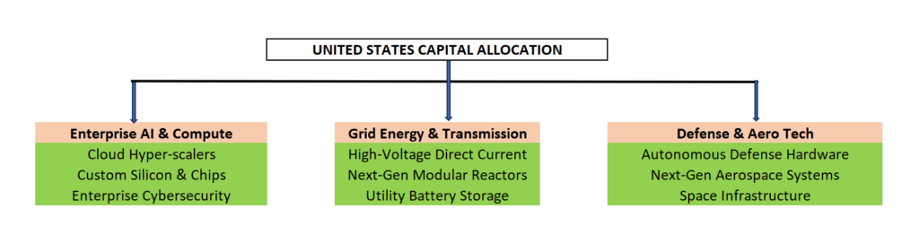
- Enterprise AI, Cloud Compute, & Cybersecurity: Companies building enterprise-grade software, AI agents, cloud architectures, and specialized hardware protection layers.
- Next-Generation Energy & Grid Modernization: Power generation utilities, high-voltage electrical equipment makers, small modular nuclear reactor (SMR) developers, and energy storage systems catering to exponential data center energy demands.
- Advanced Defense Technology & Aerospace: Autonomous systems, satellite networks, hypersonic defense, and advanced materials supplying both domestic security needs and global allied demand.
Strategic Summary for Global Investors & Executives
The United States through 2030 remains the ultimate high-volume, high-yield destination for institutional capital. While fiscal debt risks require long-term monitoring, the immediate 5-year outlook is defined by strong technology-driven productivity, resilient private consumption, and unmatched market liquidity. For global corporations and institutional allocators, exposure to the US economy remains an indispensable pillar of long-term growth strategy.
Top 65 Largest Economies in the World for 2027
Top 10 Largest Economies by 2030: IMF & World Bank GDP Projections for Global Powerhouses

U.S.- Canada Trade Talks Collapse; Carney Says Retaliatory Tariffs Begin September 8

Flock Cameras and the Future of Public Security

AI Infrastructure Boom Hits Physical Limits: Power, Financing, and Supply Chain Strain

Armanino adds Strategic Accounting Outsourced Solutions

New 2023 K-1 instructions stir the CAMT pot for partnerships and corporations

Tax Strategy: Employee Retention Credit update
-

 Stock News1 week ago
Nvidia Earnings Preview: What Wall Street Expects From the AI Bellwether’s Q2 Report
-

 Accounting1 week ago
SEC’s Semiannual Reporting Proposal Faces Investor Pushback: What CFOs Need to Know
-

 Stock News1 week ago
Nvidia Q2 FY2027 Earnings beats Wall Street Expectation with Record $96.2 Billion Revenue
-

 Finance1 week ago
Treasury Bond Volatility Forces Bessent to Double Debt Buyback Size as Yields Swing
-
 Technology5 days ago
AI Infrastructure Boom Hits Physical Limits: Power, Financing, and Supply Chain Strain
-
 Technology3 days ago
Flock Cameras and the Future of Public Security
-
 Economics3 days ago
U.S.- Canada Trade Talks Collapse; Carney Says Retaliatory Tariffs Begin September 8